Sentiment Analysis in R

Introduction

This tutorial introduces Sentiment Analysis (SA) in R — a powerful method for extracting information about emotion and opinion from natural language (Silge and Robinson 2017). We’ll use modern R packages including sentimentr (Rinker 2021) and tidytext (Silge and Robinson 2016), along with the Word-Emotion Association Lexicon (Mohammad and Turney 2013).

Learning Outcomes

By the end of this tutorial, you will be able to:

1. Understand the principles of sentiment analysis and its applications in linguistics
   
2. Perform basic sentiment analysis using the Word-Emotion Association Lexicon
   
3. Calculate polarity ratios and emotion scores from text data
   
4. Visualize sentiment patterns across texts and over narrative time
   
5. Identify key emotive words contributing to sentiment scores
   
6. Track changes in sentiment using binning and rolling averages
   
7. Apply context-sensitive sentiment analysis that accounts for negation

---

What Is Sentiment Analysis?

Sentiment Analysis (SA) is a computational method for extracting information about emotion, opinion, or attitude from natural language (Silge and Robinson 2017). SA has been successfully applied across disciplines including psychology, economics, education, political science, and social sciences.

Why Use Sentiment Analysis?

SA offers several advantages over traditional methods:

✓ Fully replicable: Emotion coding is automated and consistent
✓ Scalable: Can analyze thousands of documents quickly
✓ Quantitative: Produces numerical scores for statistical analysis
✓ Unobtrusive: Can analyze existing text without surveys or experiments

Beyond Simple Polarity

Many SA tools provide only polarity (positive vs. negative). However, linguistics research often requires more nuanced information. This tutorial uses the Word-Emotion Association Lexicon, which provides scores for eight core emotions:

Emotion	Example Words
Joy	happy, beautiful, wonderful
Trust	safe, honest, reliable
Anticipation	ready, hope, expect
Surprise	wow, sudden, amazing
Sadness	cry, tragedy, loss
Fear	afraid, terror, panic
Disgust	sick, ugly, awful
Anger	fit, burst, hate

This fine-grained approach allows us to investigate specific emotional dimensions rather than just crude positive-negative distinctions.

---

Prerequisites

Required Background

Before starting this tutorial, we recommend familiarity with:

• Getting started with R
  
• String Processing in R
  
• Data manipulation with tidyverse
  
• Basic data visualization with ggplot2

---

The Word-Emotion Association Lexicon

The Word-Emotion Association Lexicon (Mohammad and Turney 2013) comprises 10,170 terms with emotion associations based on crowd-sourced ratings from Amazon Mechanical Turk:

• 38,726 ratings from 2,216 raters
  
• Each term rated 5 times
  
• 85% of words had 4+ identical ratings (high reliability)

How it works: Raters were asked whether each word was associated with one or more of eight emotions. The resulting associations are highly reliable and capture intuitive emotional connotations.

Example Associations

• cry, tragedy → SADNESS
  
• happy, beautiful → JOY
  
• fit, burst → ANGER
  
• safe, friend → TRUST

---

Preparation and Setup

Install Packages

If you haven’t already installed the required packages:

install.packages(c("tidyverse", "tidytext", "sentimentr", "Hmisc",  
                   "zoo", "flextable", "checkdown"))  

Load Packages

library(tidyverse)   # data manipulation & ggplot2  
library(tidytext)    # text mining  
library(sentimentr)  # context-sensitive sentiment  
library(Hmisc)       # binning with cut2()  
library(zoo)         # rolling means with rollapply()  
library(flextable)   # formatted tables  
library(checkdown)   # interactive exercises  
  
options(stringsAsFactors = FALSE)  
options(scipen = 999)  

Load Example Data

We’ll analyze four classic texts to demonstrate sentiment analysis:

# load texts  
darwin <- base::readRDS(here::here("tutorials/sentiment/data", "origindarwin.rda"))  
twain <- base::readRDS(here::here("tutorials/sentiment/data", "twainhuckfinn.rda"))  
orwell <- base::readRDS(here::here("tutorials/sentiment/data", "orwell.rda"))  
lovecraft <- base::readRDS(here::here("tutorials/sentiment/data", "lovecraftcolor.rda"))  

head(darwin, 10)
THE ORIGIN OF SPECIES
BY
CHARLES DARWIN
AN HISTORICAL SKETCH
OF THE PROGRESS OF OPINION ON
THE ORIGIN OF SPECIES
INTRODUCTION
When on board H.M.S. 'Beagle,' as naturalist, I was much struck
with certain facts in the distribution of the organic beings in-
habiting South America, and in the geological relations of the

---

Part I: Basic Sentiment Analysis

Text Preprocessing

Before sentiment analysis, we need to clean and tokenize the texts.

Create Cleaning Function

# function to clean and tokenize text  
txtclean <- function(x, title) {  
  x |>  
    # convert to UTF-8 encoding  
    iconv(to = "UTF-8") |>  
    # lowercase  
    base::tolower() |>  
    # collapse into single string  
    paste0(collapse = " ") |>  
    # remove extra whitespace  
    stringr::str_squish() |>  
    # split into words  
    stringr::str_split(" ") |>  
    unlist() |>  
    # convert to tibble  
    tibble::tibble() |>  
    # rename column  
    dplyr::select(word = 1, everything()) |>  
    # add novel identifier  
    dplyr::mutate(novel = title) |>  
    # remove stopwords (the, a, an, etc.)  
    dplyr::anti_join(tidytext::stop_words, by = "word") |>  
    # remove non-alphabetic characters  
    dplyr::mutate(word = stringr::str_remove_all(word, "\\W")) |>  
    # remove empty strings  
    dplyr::filter(word != "")  
}  

Why Remove Stopwords?

Stopwords (e.g., the, a, an, of) are high-frequency function words with little semantic content. Removing them:

• Reduces noise in sentiment analysis
  
• Focuses on content words (nouns, verbs, adjectives)
  
• Improves computational efficiency

However: For context-sensitive analysis (Part III), we’ll keep stopwords because negators like not and never affect sentiment.

Clean All Texts

# process all four texts  
darwin_clean <- txtclean(darwin, "darwin")  
lovecraft_clean <- txtclean(lovecraft, "lovecraft")  
orwell_clean <- txtclean(orwell, "orwell")  
twain_clean <- txtclean(twain, "twain")  

word	novel
origin	darwin
species	darwin
charles	darwin
darwin	darwin
historical	darwin
sketch	darwin
progress	darwin
opinion	darwin
origin	darwin
species	darwin

---

Perform Sentiment Analysis

Now we join the cleaned texts with the Word-Emotion Association Lexicon:

Citation Note

If you use the Word-Emotion Association Lexicon (NRC), please cite

Mohammad, Saif M, and Peter D Turney. 2013. Crowdsourcing a Word-Emotion Association Lexicon. Computational Intelligence 29 (3): 436–65. https://doi.org/https://doi.org/10.1111/j.1467-8640.2012.00460.x.

nrc <- tidytext::get_sentiments(lexicon = "nrc")

# combine texts and join with sentiment lexicon  
novels_anno <- rbind(darwin_clean, twain_clean, orwell_clean, lovecraft_clean) |>  
  dplyr::group_by(novel) |>  
  # count total words per novel  
  dplyr::mutate(words = n()) |>  
  # join with sentiment lexicon  
  dplyr::left_join(nrc, by = "word", relationship =
  "many-to-many") |>  
  dplyr::mutate(  
    novel = factor(novel),  
    sentiment = factor(sentiment)  
  )  

word	novel	words	sentiment
origin	darwin	76,710
species	darwin	76,710
charles	darwin	76,710
darwin	darwin	76,710
historical	darwin	76,710
sketch	darwin	76,710
progress	darwin	76,710	anticipation
progress	darwin	76,710	joy
progress	darwin	76,710	positive
opinion	darwin	76,710

Interpreting the Results

• word: The token from the text
  
• novel: Which text it came from
  
• words: Total word count for that novel
  
• sentiment: Associated emotion (NA if word not in lexicon)

Words not in the NRC lexicon receive NA for sentiment (neutral/unassociated).

---

Calculate Emotion Frequencies

Summarize sentiment frequencies and calculate percentages:

novels <- novels_anno |>  
  dplyr::group_by(novel, sentiment) |>  
  dplyr::summarise(  
    sentiment_freq = n(),  
    words = unique(words),  
    .groups = "drop"  
  ) |>  
  # remove NA sentiments  
  dplyr::filter(!is.na(sentiment)) |>  
  # calculate percentage of emotive words  
  dplyr::mutate(percentage = round(sentiment_freq / words * 100, 1))  

novel	sentiment	sentiment_freq	words	percentage
darwin	anger	1,255	76,710	1.6
darwin	anticipation	2,291	76,710	3.0
darwin	disgust	851	76,710	1.1
darwin	fear	2,236	76,710	2.9
darwin	joy	1,754	76,710	2.3
darwin	negative	4,294	76,710	5.6
darwin	positive	6,469	76,710	8.4
darwin	sadness	2,050	76,710	2.7
darwin	surprise	1,239	76,710	1.6
darwin	trust	3,955	76,710	5.2
lovecraft	anger	197	4,847	4.1
lovecraft	anticipation	184	4,847	3.8
lovecraft	disgust	173	4,847	3.6
lovecraft	fear	288	4,847	5.9
lovecraft	joy	106	4,847	2.2

---

Visualize Emotion Profiles

Plot Emotions by Novel

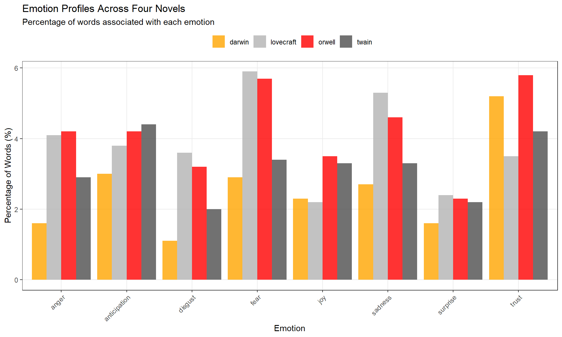
# plot 8 core emotions (exclude positive/negative polarity)  
novels |>  
  dplyr::filter(  
    sentiment != "positive",  
    sentiment != "negative"  
  ) |>  
  ggplot(aes(sentiment, percentage, fill = novel)) +  
  geom_col(position = position_dodge(), alpha = 0.8) +  
  scale_fill_manual(  
    name = "",  
    values = c("orange", "gray70", "red", "grey30")  
  ) +  
  theme_bw() +  
  labs(  
    title = "Emotion Profiles Across Four Novels",  
    subtitle = "Percentage of words associated with each emotion",  
    x = "Emotion", y = "Percentage of Words (%)"  
  ) +  
  theme(  
    legend.position = "top",  
    panel.grid.minor = element_blank(),  
    axis.text.x = element_text(angle = 45, hjust = 1)  
  )  

Plot Novels by Emotion

Reorder emotions from negative (red) to positive (blue):

novels |>  
  dplyr::filter(  
    sentiment != "positive",  
    sentiment != "negative"  
  ) |>  
  dplyr::mutate(  
    sentiment = factor(sentiment, levels = c(  
      "anger", "fear", "disgust", "sadness",  
      "surprise", "anticipation", "trust", "joy"  
    ))  
  ) |>  
  ggplot(aes(novel, percentage, fill = sentiment)) +  
  geom_col(position = position_dodge(), alpha = 0.9) +  
  scale_fill_brewer(palette = "RdBu", name = "Emotion") +  
  theme_bw() +  
  labs(  
    title = "Emotion Comparison by Novel",  
    subtitle = "Ordered from negative (red) to positive (blue)",  
    x = "", y = "Percentage of Words (%)"  
  ) +  
  theme(legend.position = "right") +  
  coord_flip()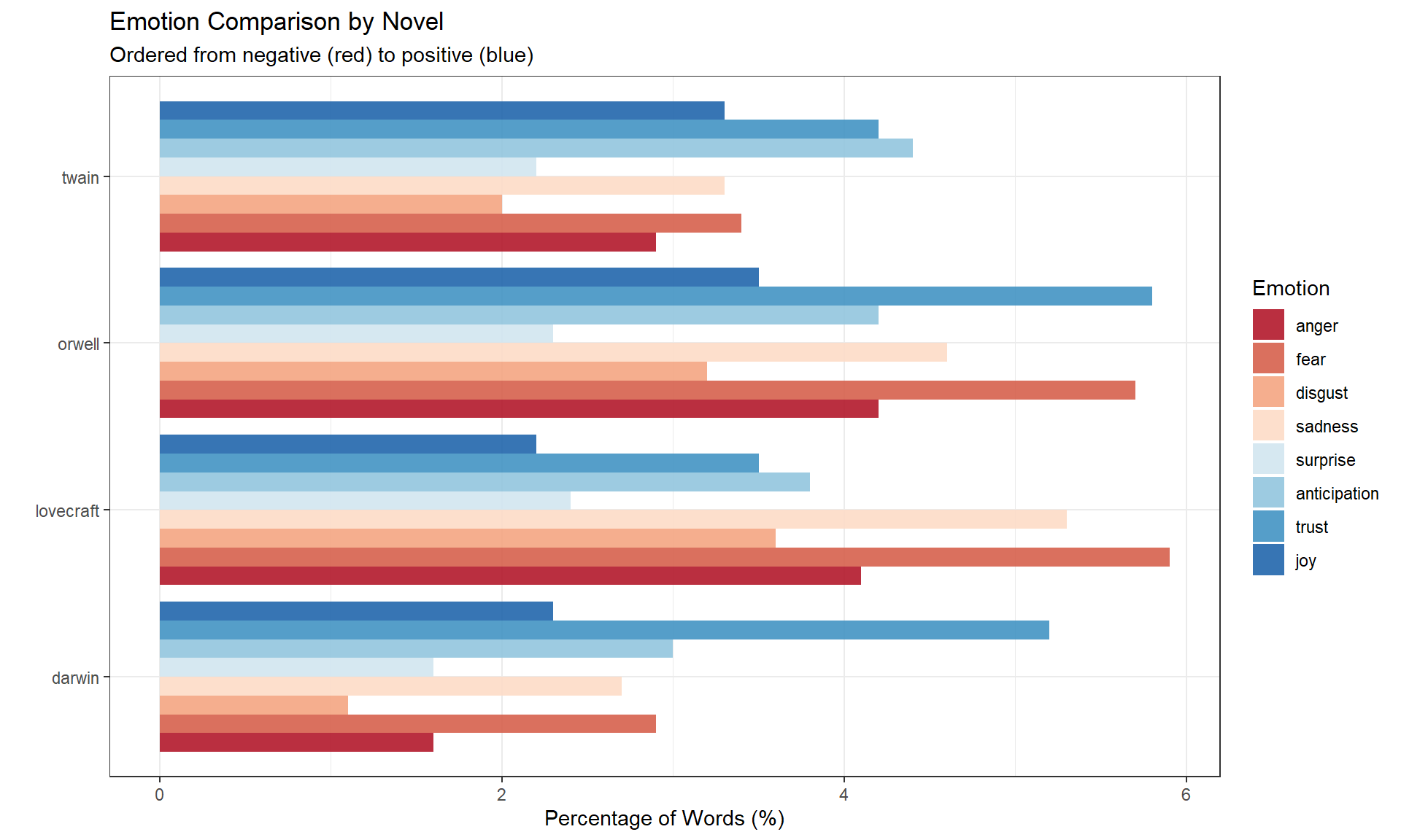  

---

Exercises: Basic Sentiment Analysis

Q1. What does it mean if a novel has 5% “joy” words?

The novel is 5% positive overall
5% of emotive words (excluding neutral) express joy
5% of all sentences express joy
5% of all words in the novel are associated with joy in the NRC lexicon

---

Q2. Why do we remove stopwords before sentiment analysis?

Stopwords are high-frequency function words (the, a, of) with little emotional content — removing them reduces noise
The NRC lexicon doesn't include stopwords
Removing stopwords is required for all text analysis in R
Stopwords are always negative and would skew results

---

Part II: Identifying Important Emotives

Which specific words contribute most to each emotion category? Let’s find the top emotive words.

Extract Top Emotive Words

We’ll focus on four emotions for clarity:

novels_impw <- novels_anno |>  
  dplyr::filter(  
    !is.na(sentiment),  
    # focus on 4 core emotions  
    sentiment %in% c("anger", "fear", "trust", "joy")  
  ) |>  
  # order emotions from negative to positive  
  dplyr::mutate(  
    sentiment = factor(sentiment, levels = c("anger", "fear", "trust", "joy"))  
  ) |>  
  dplyr::group_by(novel, sentiment) |>  
  # count word frequencies by sentiment  
  dplyr::count(word, sort = TRUE) |>  
  # get top 3 words per novel × sentiment combination  
  dplyr::top_n(3, n) |>  
  # calculate proportion within each group  
  dplyr::mutate(score = n / sum(n)) |>  
  dplyr::ungroup()  

novel	sentiment	word	n	score
darwin	trust	structure	243	0.4308511
darwin	trust	found	166	0.2943262
darwin	joy	found	166	0.4649860
darwin	trust	theory	155	0.2748227
twain	trust	pretty	148	0.4327485
twain	joy	pretty	148	0.4327485
orwell	fear	war	114	0.4710744
darwin	fear	doubt	106	0.3486842
darwin	fear	change	102	0.3355263
darwin	joy	perfect	100	0.2801120
darwin	anger	difficulty	96	0.4120172
darwin	fear	difficulty	96	0.3157895
darwin	joy	organ	91	0.2549020
darwin	anger	struggle	80	0.3433476
twain	trust	found	72	0.2105263

Visualize Top Emotive Words

novels_impw |>  
  dplyr::group_by(novel) |>  
  # get top 20 words overall  
  dplyr::slice_max(score, n = 20) |>  
  dplyr::arrange(desc(score)) |>  
  dplyr::ungroup() |>  
  ggplot(aes(x = reorder(word, score), y = score, fill = word)) +  
  facet_wrap(novel ~ sentiment, ncol = 4, scales = "free_y") +  
  geom_col(show.legend = FALSE, alpha = 0.8) +  
  coord_flip() +  
  theme_bw() +  
  labs(  
    title = "Top Emotive Words by Novel and Emotion",  
    subtitle = "Showing most frequent emotion-associated words",  
    x = "Word", y = "Proportion within emotion category"  
  ) +  
  theme(  
    strip.text = element_text(face = "bold"),  
    panel.grid.minor = element_blank()  
  )  

Interpreting the Visualization

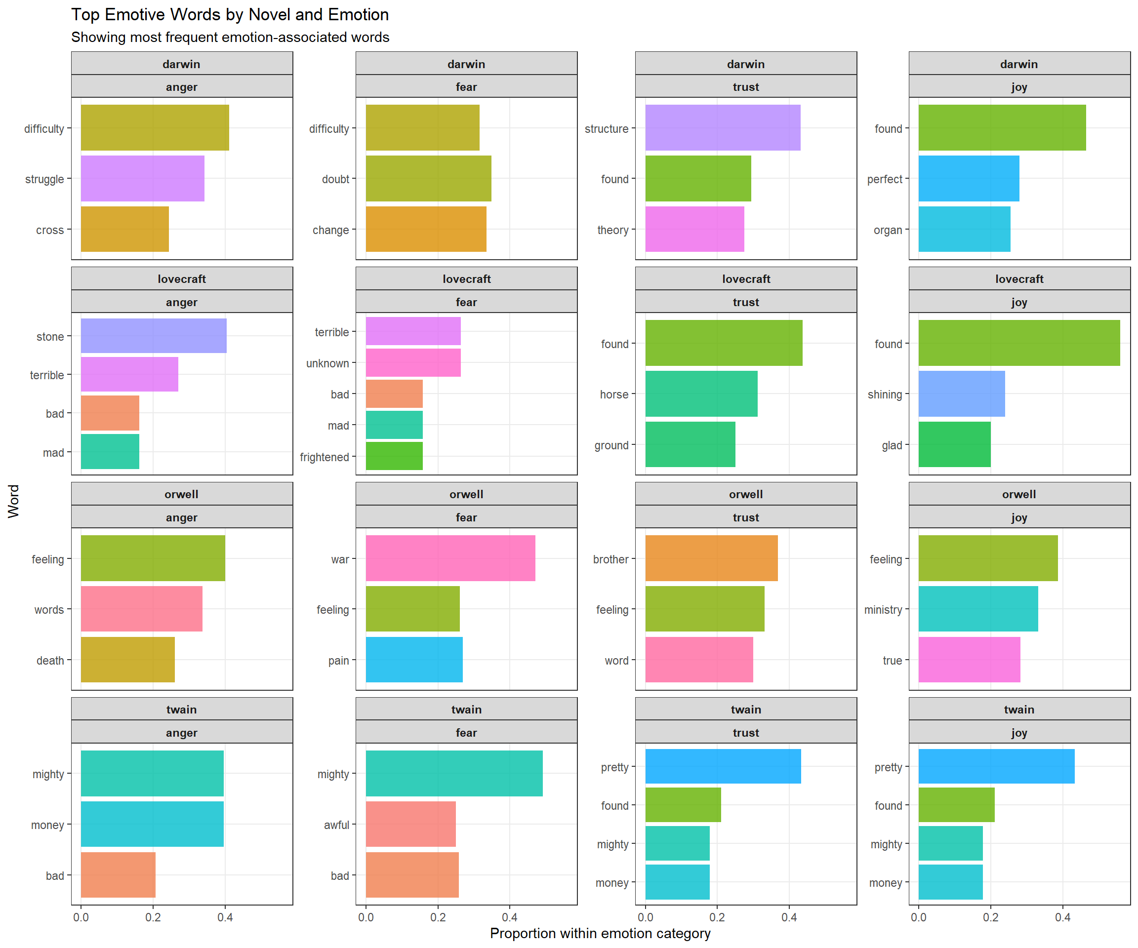
Each panel shows the top words for a specific novel × emotion combination. For example:

• Darwin + Trust: Words like nature, species, selection reflect scientific confidence
  
• Lovecraft + Fear: Words like horror, terrible, dread reflect the horror genre
  
• Orwell + Anger: Words like hate, war, enemy reflect dystopian themes

This reveals genre-specific emotion vocabularies.

---

Part III: Polarity Analysis

Polarity measures the ratio of positive to negative emotion words. It’s a simple but powerful metric for overall emotional tone.

Calculate Polarity Ratios

polarity_scores <- novels |>  
  # keep only positive/negative tags  
  dplyr::filter(sentiment %in% c("positive", "negative")) |>  
  dplyr::select(novel, sentiment, sentiment_freq) |>  
  # pivot wider for calculation  
  tidyr::pivot_wider(  
    names_from = sentiment,  
    values_from = sentiment_freq,  
    values_fill = 0  
  ) |>  
  # calculate polarity ratio  
  dplyr::mutate(polarity = positive / negative)  

novel	negative	positive	polarity
darwin	4,294	6,469	1.5065207
lovecraft	526	318	0.6045627
orwell	3,455	3,425	0.9913169
twain	1,892	2,386	1.2610994

Visualize Polarity

polarity_scores |>  
  ggplot(aes(x = reorder(novel, polarity), y = polarity, fill = novel)) +  
  geom_col(alpha = 0.8, show.legend = FALSE) +  
  geom_text(  
    aes(y = polarity - 0.1, label = round(polarity, 2)),  
    color = "white", size = 5, fontface = "bold"  
  ) +  
  geom_hline(yintercept = 1, linetype = "dashed", color = "gray30") +  
  theme_bw() +  
  labs(  
    title = "Polarity Comparison Across Novels",  
    subtitle = "Ratio of positive to negative emotion words",  
    y = "Polarity Ratio\n(positive ÷ negative)",  
    x = ""  
  ) +  
  scale_y_continuous(  
    breaks = c(0, 1, 2),  
    labels = c("More negative", "Neutral", "More positive")  
  ) +  
  coord_cartesian(y = c(0, 2.5)) +  
  theme(panel.grid.minor = element_blank())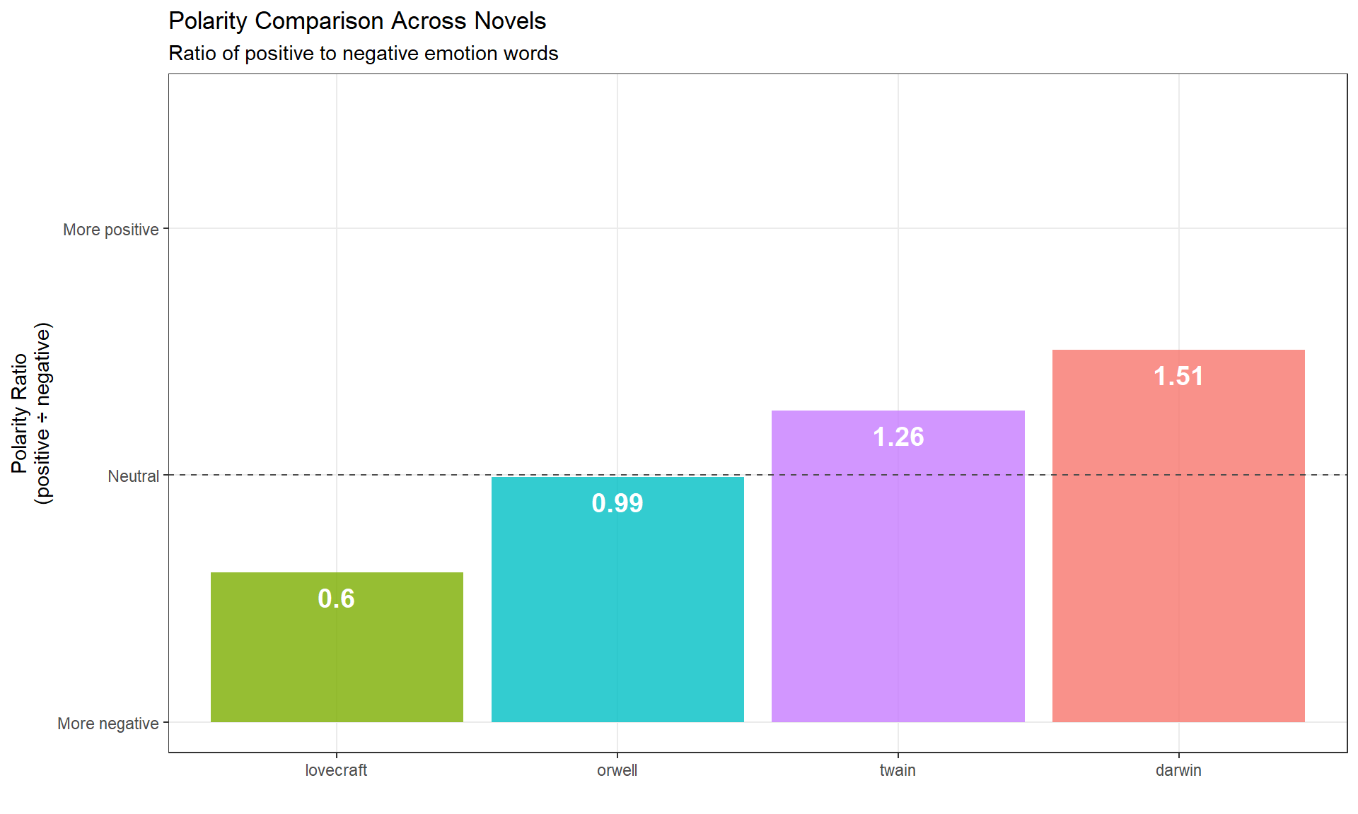  

Interpreting Polarity

• Polarity = 1: Equal positive and negative words (neutral)
  
• Polarity > 1: More positive than negative (optimistic tone)
  
• Polarity < 1: More negative than positive (pessimistic tone)

All four novels have polarity > 1 (more positive than negative), but Lovecraft is closest to neutral, reflecting its horror/dark themes.

---

Exercises: Polarity Analysis

Q1. A novel has 800 positive emotion words and 400 negative emotion words. What is its polarity ratio?

0.5 (= 400 ÷ 800) — half as many negative as positive
1200 (= 800 + 400) — total emotive words
400 (= 800 − 400) — net positive difference
2.0 (= 800 ÷ 400) — twice as many positive as negative

---

Q2. What does a polarity ratio of 0.8 indicate?

The difference between positive and negative is 0.8 words
Exactly 80% of words are positive
More negative than positive words — the text has a pessimistic tone
More positive than negative words — the text has an optimistic tone

---

Part IV: Tracking Changes Over Time

How does sentiment change as a narrative unfolds? We’ll use two methods: binning and rolling averages.

Method 1: Binning

Binning divides text into equal-sized chunks and calculates sentiment within each bin.

Prepare Data for Binning

novels_bin <- novels_anno |>  
  dplyr::group_by(novel) |>  
  # keep only polarity tags  
  dplyr::filter(is.na(sentiment) | sentiment %in% c("negative", "positive")) |>  
  # convert to numeric: positive = +1, negative = −1, neutral = 0  
  dplyr::mutate(  
    sentiment = as.character(sentiment),  
    sentiment = case_when(  
      is.na(sentiment) ~ "0",  
      TRUE ~ sentiment  
    ),  
    sentiment = case_when(  
      sentiment == "0" ~ 0,  
      sentiment == "positive" ~ 1,  
      TRUE ~ -1  
    ),  
    # create word index  
    id = 1:n(),  
    # divide into bins of 100 words each  
    index = as.numeric(Hmisc::cut2(id, m = 100))  
  ) |>  
  dplyr::group_by(novel, index) |>  
  # calculate mean polarity per bin  
  dplyr::summarize(  
    polarity = mean(sentiment),  
    .groups = "drop"  
  )  

novel	index	polarity
darwin	1	0.03960396
darwin	2	0.12000000
darwin	3	0.11000000
darwin	4	0.09000000
darwin	5	0.01000000
darwin	6	0.11000000
darwin	7	0.03000000
darwin	8	0.08000000
darwin	9	0.04000000
darwin	10	0.01000000
darwin	11	0.01000000
darwin	12	0.03000000
darwin	13	-0.03000000
darwin	14	0.04000000
darwin	15	0.09000000

How Binning Works

1. Assign numeric values: positive = +1, negative = −1, neutral = 0
   
2. Divide text into bins: e.g., bin 1 = words 1–100, bin 2 = 101–200, etc.
   
3. Calculate mean: Average sentiment value within each bin
   
4. Plot over time: Show how polarity changes across bins

Bin size matters: Too small = noisy; too large = loses detail. 100 words is typical.

Visualize Sentiment Trajectories

ggplot(novels_bin, aes(index, polarity)) +  
  facet_wrap(~ novel, scales = "free_x", ncol = 2) +  
  geom_line(alpha = 0.3, color = "gray50") +  
  geom_smooth(se = TRUE, color = "steelblue", fill = "lightblue") +  
  geom_hline(yintercept = 0, linetype = "dashed", color = "red") +  
  theme_bw() +  
  labs(  
    title = "Sentiment Trajectories Across Narratives (Binning Method)",  
    subtitle = "Smoothed trend with 95% confidence interval",  
    y = "Polarity (mean by bin)",  
    x = "Narrative progression (bin index)"  
  ) +  
  theme(  
    strip.text = element_text(face = "bold", size = 11),  
    panel.grid.minor = element_blank()  
  )  

`geom_smooth()` using method = 'loess' and formula = 'y ~ x'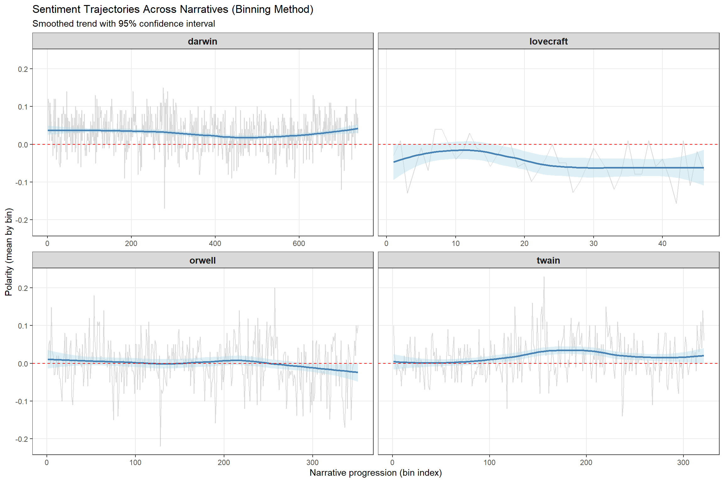

Interpreting Trajectories

• Above zero: Positive polarity dominates in that section
  
• Below zero: Negative polarity dominates
  
• Slope: Rising = becoming more positive; falling = becoming more negative

For example, if Orwell’s 1984 shows declining polarity toward the end, this reflects the increasingly dystopian/pessimistic narrative arc.

---

Method 2: Rolling Averages

Rolling averages (also called moving averages) calculate the mean within a sliding window.

Binning vs. Rolling Averages

• Binning: Divides text into non-overlapping chunks → shows discrete changes
  
• Rolling averages: Sliding window → smooths fluctuations, better for trends

Rolling averages are NOT ideal for tracking changes — they smooth data too much. Use binning to detect actual shifts; use rolling averages to visualize overall trends.

Calculate Rolling Means

novels_change <- novels_anno |>
  # keep only polarity
  dplyr::filter(is.na(sentiment) | sentiment %in% c("negative", "positive")) |>
  dplyr::group_by(novel) |>
  # convert to numeric
  dplyr::mutate(
    sentiment = as.character(sentiment),
    sentiment = case_when(
      is.na(sentiment) ~ "0",
      TRUE ~ sentiment
    ),
    sentiment = case_when(
      sentiment == "0" ~ 0,
      sentiment == "positive" ~ 1,
      TRUE ~ -1
    ),
    id = 1:n()
  ) |>
  dplyr::reframe(
    id = id,
    # rolling mean with window = 100 words
    rmean = zoo::rollapply(
      sentiment, 
      width = 100, 
      FUN = mean, 
      align = "right", 
      fill = NA
    )
  ) |>
  na.omit()

novel	id	rmean
darwin	100	0.04
darwin	101	0.04
darwin	102	0.04
darwin	103	0.04
darwin	104	0.04
darwin	105	0.04
darwin	106	0.04
darwin	107	0.04
darwin	108	0.04
darwin	109	0.04
darwin	110	0.04
darwin	111	0.04
darwin	112	0.04
darwin	113	0.04
darwin	114	0.03

Visualize Rolling Averages

ggplot(novels_change, aes(id, rmean)) +  
  facet_wrap(~ novel, scales = "free_x", ncol = 2) +  
  geom_line(alpha = 0.5, color = "steelblue") +  
  geom_smooth(se = F, color = "darkblue", fill = "lightblue", method = "loess") +  
  geom_hline(yintercept = 0, linetype = "dashed", color = "red") +  
  theme_bw() +  
  labs(  
    title = "Sentiment Trajectories Using Rolling Averages",  
    subtitle = "Window = 100 words",  
    y = "Polarity (rolling mean, k = 100)",  
    x = "Word position in text"  
  ) +  
  theme(  
    strip.text = element_text(face = "bold", size = 11),  
    panel.grid.minor = element_blank()  
  )  

`geom_smooth()` using formula = 'y ~ x'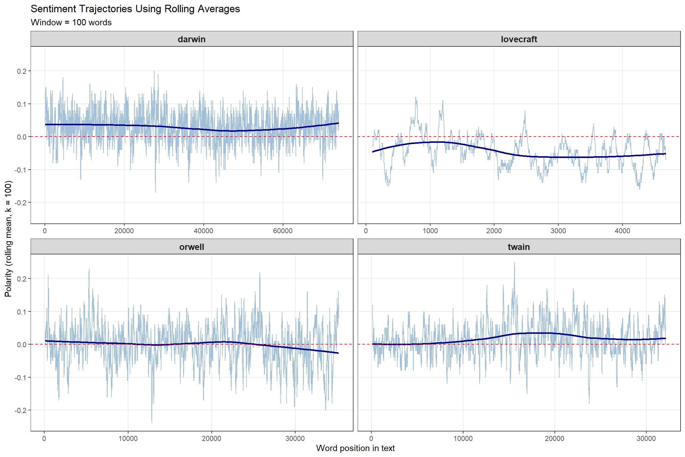

---

Exercises: Tracking Changes

Q1. What is the main difference between binning and rolling averages?

They produce identical results but use different code
Rolling averages are always more accurate than binning
Binning uses non-overlapping chunks; rolling averages use overlapping sliding windows
Binning calculates means; rolling averages calculate medians

---

Q2. Why is binning generally preferred over rolling averages for detecting sentiment changes in narratives?

Rolling averages require more computational power
Rolling averages only work for positive sentiment
Binning works with any window size; rolling averages require exactly 100 words
Binning preserves discrete shifts in sentiment; rolling averages over-smooth and obscure changes

---

Part V: Context-Sensitive Sentiment Analysis

So far, we’ve ignored how context affects meaning. The sentence “You are a good boy” and “You are not a good boy” would receive identical scores because we removed stopwords including negators.

In this section, we incorporate negation using the sentimentr package, which accounts for words like not, never, neither that reverse polarity.

Limitation

We focus on polarity only (positive/negative), not the 8 core emotions. Context-sensitive emotion analysis would require a custom sentiment lexicon with negation rules for each emotion.

Prepare Sentences

We’ll analyze the first 50 sentences from Orwell’s 1984:

# split into sentences  
orwell_sent <- orwell |>  
  iconv(to = "latin1") |>  
  paste0(collapse = " ") |>  
  # remove hyphenation  
  stringr::str_replace_all("([a-z])- ([a-z])", "\\1\\2") |>  
  stringr::str_squish() |>  
  tibble::tibble() |>  
  dplyr::select(text = 1) |>  
  # tokenize by sentences  
  tidytext::unnest_tokens(sentence, text, token = "sentences") |>  
  # keep first 50 sentences  
  dplyr::slice_head(n = 50)  

sentence
1984 george orwell part 1, chapter 1 it was a bright cold day in april, and the clocks were striking thirteen.
winston smith, his chin nuzzled into his breast in an effort to escape the vile wind, slipped quickly through the glass doors of victory mansions, though not quickly enough to prevent a swirl of gritty dust from entering along with him.
the hallway smelt of boiled cabbage and old rag mats.
at one end of it a coloured poster, too large for indoor display, had been tacked to the wall.
it depicted simply an enormous face, more than a metre wide: the face of a man of about forty-five, with a heavy black moustache and ruggedly handsome features.
winston made for the stairs.
it was no use trying the lift.
even at the best of times it was seldom working, and at present the electric current was cut off during daylight hours.
it was part of the economy drive in preparation for hate week.
the flat was seven flights up, and winston, who was thirty-nine and had a varicose ulcer above his right ankle, went slowly, resting several times on the way.

Apply Context-Sensitive SA

The sentimentr::sentiment() function accounts for:

• Negators: not, never, no
  
• Intensifiers: very, extremely, quite
  
• De-amplifiers: barely, hardly, scarcely
  
• Adversative conjunctions: but, however, although

orwell_sent_class <- orwell_sent |>  
  dplyr::mutate(  
    # calculate context-sensitive sentiment  
    sentiment_score = sentimentr::sentiment(sentence)$sentiment  
  )  

sentence	sentiment_score
1984 george orwell part 1, chapter 1 it was a bright cold day in april, and the clocks were striking thirteen.	0.11785113
winston smith, his chin nuzzled into his breast in an effort to escape the vile wind, slipped quickly through the glass doors of victory mansions, though not quickly enough to prevent a swirl of gritty dust from entering along with him.	0.21864327
the hallway smelt of boiled cabbage and old rag mats.	-0.31622777
at one end of it a coloured poster, too large for indoor display, had been tacked to the wall.	0.00000000
it depicted simply an enormous face, more than a metre wide: the face of a man of about forty-five, with a heavy black moustache and ruggedly handsome features.	0.25068871
winston made for the stairs.	0.00000000
it was no use trying the lift.	0.00000000
even at the best of times it was seldom working, and at present the electric current was cut off during daylight hours.	0.03198011
it was part of the economy drive in preparation for hate week.	-0.21650635
the flat was seven flights up, and winston, who was thirty-nine and had a varicose ulcer above his right ankle, went slowly, resting several times on the way.	-0.19498011

Interpreting Scores

• Positive scores: Sentence expresses positive sentiment
  
• Negative scores: Sentence expresses negative sentiment
  
• Magnitude: Larger absolute values = stronger sentiment

Example:
- “This is good” → +0.35
- “This is not good” → −0.35 (negation reverses polarity)
- “This is very good” → +0.50 (intensifier amplifies)

Visualize Context-Sensitive Sentiment

orwell_sent_class |>  
  dplyr::mutate(sentence_id = 1:n()) |>  
  ggplot(aes(x = sentence_id, y = sentiment_score)) +  
  geom_col(aes(fill = sentiment_score > 0), alpha = 0.8, show.legend = FALSE) +  
  geom_hline(yintercept = 0, linetype = "dashed") +  
  scale_fill_manual(values = c("red3", "steelblue")) +  
  theme_bw() +  
  labs(  
    title = "Context-Sensitive Sentiment Analysis of Orwell's 1984",  
    subtitle = "First 50 sentences (negation-aware)",  
    x = "Sentence Number", y = "Sentiment Score"  
  ) +  
  theme(panel.grid.minor = element_blank())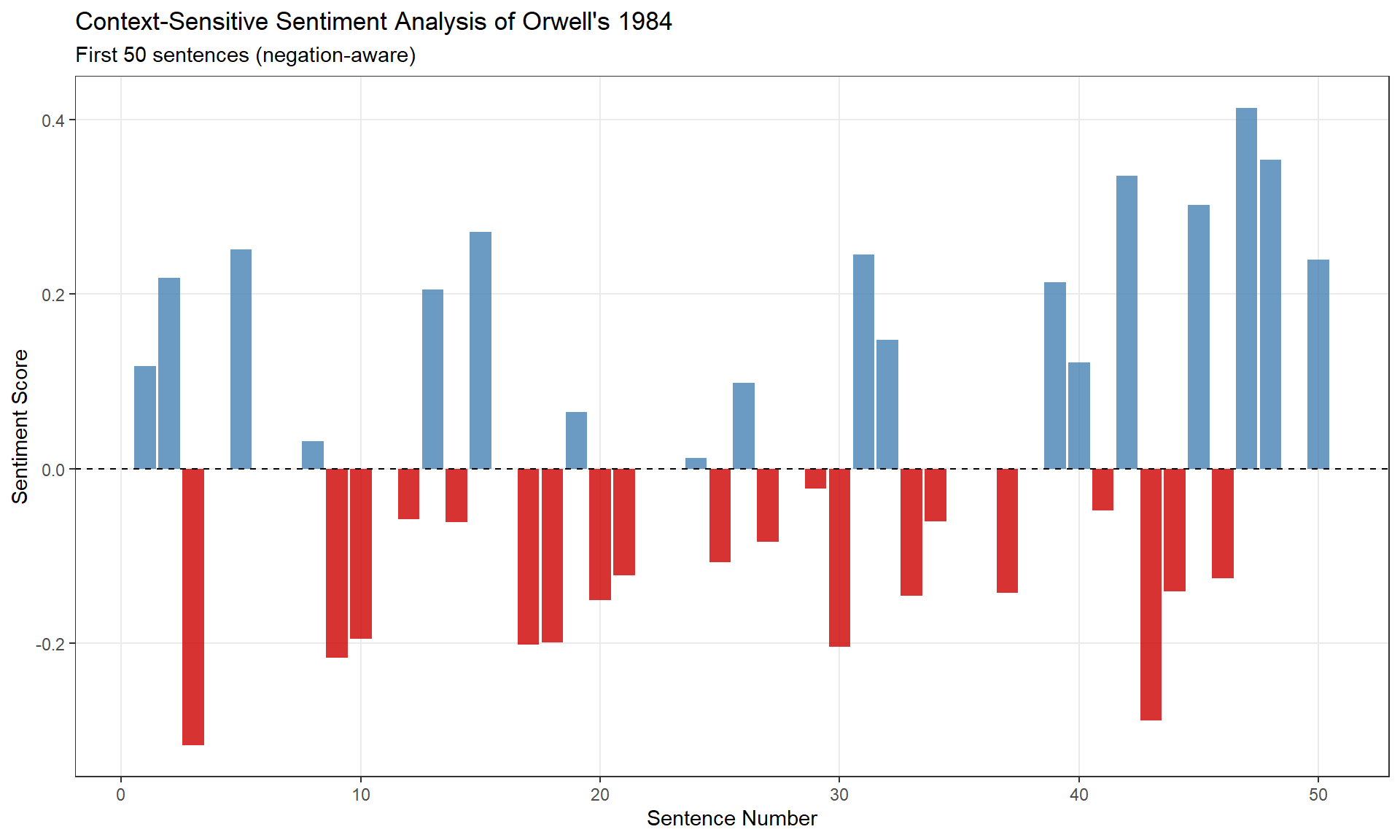  

---

Exercises: Context-Sensitive Analysis

Q1. Why does context-sensitive sentiment analysis keep stopwords instead of removing them?

Negators like 'not', 'never', 'no' are stopwords but are crucial for reversing sentiment polarity
Stopwords improve accuracy of sentiment detection
Context-sensitive analysis doesn't actually use stopwords
The sentimentr package requires stopwords to function

---

Q2. The sentence “This is not very good” receives a sentiment score of −0.45. What does this tell us?

The sentence is slightly positive (−0.45 is close to zero)
The sentence contains 45% negative words
The sentence is moderately negative — 'not' reverses 'good' and 'very' intensifies the negation
The sentiment is unreliable because the score is negative

---

Summary and Best Practices

Key Takeaways

1. Sentiment Analysis extracts emotion from text using lexicon-based methods
   
2. Word-Emotion Association Lexicon provides 8 core emotions beyond simple polarity
   
3. Polarity ratio (positive/negative) measures overall emotional tone
   
4. Binning detects discrete sentiment changes in narratives
   
5. Context-sensitive analysis accounts for negation and intensifiers

---

When to Use Each Method

Goal	Method
Compare overall emotionality of texts	Basic SA with NRC lexicon
Identify key emotive vocabulary	Top words analysis
Measure positivity/negativity	Polarity ratio
Track narrative arc changes	Binning (preferred) or rolling averages
Account for negation/intensifiers	sentimentr package

---

Limitations and Considerations

SA Limitations

1. Lexicon coverage: NRC has ~10,000 words — rare/specialized terms may be missing
   
2. Context dependence: Basic SA ignores word order, syntax, pragmatics
   
3. Domain specificity: “Sick” is negative in health contexts, positive in slang
   
4. Sarcasm/irony: Cannot detect “Oh, great, just what I needed” (sarcastic)
   
5. Cultural bias: Lexicons may reflect English/Western emotional norms

Always validate results with close reading and domain expertise.

---

Further Reading

For more advanced sentiment analysis:

• Silge and Robinson (2017): Text Mining with R (free online: tidytextmining.com)
  
• Mohammad and Turney (2013): Original NRC lexicon paper
  
• sentimentr documentation: Context-sensitive methods
  
• syuzhet package: Narrative trajectory analysis

---

AI Usage Statement

Use of AI in Tutorial Development

This tutorial was developed with assistance from Claude (Anthropic) for:

✓ Structuring content and creating callout boxes
✓ Generating interactive checkdown exercises
✓ Writing clear explanations of statistical concepts
✓ Creating modern ggplot2 visualizations
✓ Improving code documentation and comments

All code examples were tested, all statistical content was verified against published sources, and all pedagogical decisions were made by the tutorial author (Martin Schweinberger).

---

Citation & Session Info

Schweinberger, Martin. 2026. Sentiment Analysis in R. Brisbane: The University of Queensland. url: https://ladal.edu.au/tutorials/sentiment/sentiment.html (Version 2026.02.24).

@manual{schweinberger2026sentiment,  
  author = {Schweinberger, Martin},  
  title = {Sentiment Analysis in R},  
  note = {https://ladal.edu.au/tutorials/sentiment/sentiment.html},  
  year = {2026},  
  organization = {The University of Queensland, School of Languages and Cultures},  
  address = {Brisbane},  
  edition = {2026.02.24}  
}  

sessionInfo()  

R version 4.4.2 (2024-10-31 ucrt)
Platform: x86_64-w64-mingw32/x64
Running under: Windows 11 x64 (build 26200)

Matrix products: default


locale:
[1] LC_COLLATE=English_United States.utf8 
[2] LC_CTYPE=English_United States.utf8   
[3] LC_MONETARY=English_United States.utf8
[4] LC_NUMERIC=C                          
[5] LC_TIME=English_United States.utf8    

time zone: Australia/Brisbane
tzcode source: internal

attached base packages:
[1] stats     graphics  grDevices datasets  utils     methods   base     

other attached packages:
 [1] lubridate_1.9.4  forcats_1.0.0    purrr_1.0.4      readr_2.1.5     
 [5] tidyverse_2.0.0  checkdown_0.0.13 syuzhet_1.0.7    zoo_1.8-13      
 [9] tidytext_0.4.2   tidyr_1.3.2      tibble_3.2.1     textdata_0.4.5  
[13] stringr_1.5.1    sentimentr_2.9.0 Hmisc_5.2-2      ggplot2_4.0.2   
[17] flextable_0.9.11 dplyr_1.2.0     

loaded via a namespace (and not attached):
 [1] tidyselect_1.2.1        farver_2.1.2            S7_0.2.1               
 [4] fastmap_1.2.0           textshape_1.7.5         fontquiver_0.2.1       
 [7] janeaustenr_1.0.0       digest_0.6.39           rpart_4.1.23           
[10] timechange_0.3.0        lifecycle_1.0.5         cluster_2.1.6          
[13] tokenizers_0.3.0        magrittr_2.0.3          compiler_4.4.2         
[16] rlang_1.1.7             tools_4.4.2             yaml_2.3.10            
[19] qdapRegex_0.7.8         data.table_1.17.0       knitr_1.51             
[22] labeling_0.4.3          askpass_1.2.1           htmlwidgets_1.6.4      
[25] xml2_1.3.6              textclean_0.9.3         RColorBrewer_1.1-3     
[28] withr_3.0.2             foreign_0.8-87          nnet_7.3-19            
[31] grid_4.4.2              gdtools_0.5.0           colorspace_2.1-1       
[34] scales_1.4.0            cli_3.6.4               rmarkdown_2.30         
[37] ragg_1.3.3              generics_0.1.3          rstudioapi_0.17.1      
[40] tzdb_0.4.0              commonmark_2.0.0        splines_4.4.2          
[43] base64enc_0.1-6         vctrs_0.7.1             Matrix_1.7-2           
[46] jsonlite_1.9.0          fontBitstreamVera_0.1.1 litedown_0.9           
[49] hms_1.1.3               patchwork_1.3.0         Formula_1.2-5          
[52] htmlTable_2.4.3         systemfonts_1.3.1       glue_1.8.0             
[55] codetools_0.2-20        stringi_1.8.4           gtable_0.3.6           
[58] pillar_1.10.1           htmltools_0.5.9         openssl_2.3.2          
[61] R6_2.6.1                textshaping_1.0.0       evaluate_1.0.3         
[64] lattice_0.22-6          markdown_2.0            lexicon_1.2.1          
[67] backports_1.5.0         SnowballC_0.7.1         renv_1.1.7             
[70] fontLiberation_0.1.0    Rcpp_1.1.1              zip_2.3.2              
[73] uuid_1.2-1              nlme_3.1-166            gridExtra_2.3          
[76] checkmate_2.3.2         mgcv_1.9-1              officer_0.7.3          
[79] xfun_0.56               fs_1.6.5                pkgconfig_2.0.3        

---

Back to top

Back to HOME

---

References

---

AI Transparency Statement

This tutorial was re-developed with the assistance of Claude (claude.ai), a large language model created by Anthropic. Claude was used to help revise the tutorial text, structure the instructional content, generate the R code examples, and write the checkdown quiz questions and feedback strings. All content was reviewed, edited, and approved by the author (Martin Schweinberger), who takes full responsibility for the accuracy and pedagogical appropriateness of the material. The use of AI assistance is disclosed here in the interest of transparency and in accordance with emerging best practices for AI-assisted academic content creation.

References

Mohammad, Saif M, and Peter D Turney. 2013. “Crowdsourcing a Word-Emotion Association Lexicon.” Computational Intelligence 29 (3): 436–65. https://doi.org/https://doi.org/10.1111/j.1467-8640.2012.00460.x.

Rinker, Tyler W. 2021. sentimentr: Calculate Text Polarity Sentiment. Buffalo, New York. https://github.com/trinker/sentimentr.

Silge, Julia, and David Robinson. 2016. “Tidytext: Text Mining and Analysis Using Tidy Data Principles in r.” JOSS 1 (3): 37. https://doi.org/10.21105/joss.00037.

———. 2017. Text Mining with r: A Tidy Approach. " O’Reilly Media, Inc.".